Examples
A simple example
Network definition
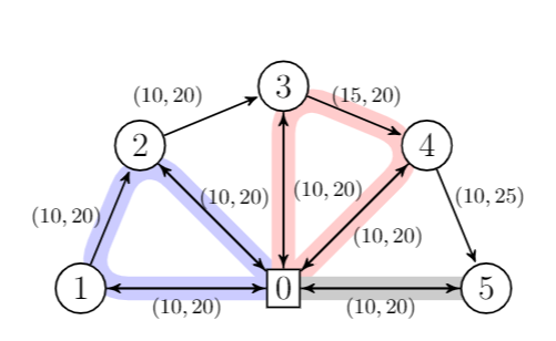
In this first example, we will be working with the following network:
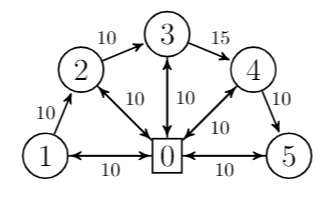
The first step is to define the network as a nx.Digraph object. Note that for convenience, the depot (node \(0\) in the picture) is split into two vertices
: the Source and the Sink.
# Create graph
>>> from networkx import DiGraph
>>> G = DiGraph()
>>> for v in [1, 2, 3, 4, 5]:
       G.add_edge("Source", v, cost=10)
       G.add_edge(v, "Sink", cost=10)
>>> G.add_edge(1, 2, cost=10)
>>> G.add_edge(2, 3, cost=10)
>>> G.add_edge(3, 4, cost=15)
>>> G.add_edge(4, 5, cost=10)
VRP definition
The second step is to define the VRP, with the above defined graph as input:
>>> from vrpy import VehicleRoutingProblem
>>> prob = VehicleRoutingProblem(G)
Maximum number of stops per route
In this first variant, it is required that a vehicle cannot perform more than \(3\) stops:
>>> prob.num_stops = 3
>>> prob.solve()
The best routes found can be queried as follows:
>>> prob.best_routes
{1: ['Source', 4, 5, 'Sink'], 2: ['Source', 1, 2, 3, 'Sink']}
And the cost of this solution is queried in a similar fashion:
>>> prob.best_value
70.0
>>> prob.best_routes_cost
{1: 30, 2: 40}
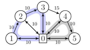
The optimal routes are displayed below:
Capacity constraints
In this second variant, we define a demand for each customer and limit the vehicle capacity to \(10\) units.
Demands are set directly as node attributes on the graph, and the capacity constraint is set with the load_capacity attribute:
>>> for v in G.nodes():
       if v not in ["Source", "Sink"]:
          G.nodes[v]["demand"] = 5
>>> prob.load_capacity = 10
>>> prob.solve()
>>> prob.best_value
80.0
As the problem is more constrained, it is not surprising that the total cost increases. As a sanity check, we can query the loads on each route to make sure capacity constraints are met:
>>> prob.best_routes
{1: ["Source", 1, "Sink"], 2: ["Source", 2, 3, "Sink"], 3: ["Source", 4, 5, "Sink"]}
>>> prob.best_routes_load
{1: 5, 2: 10, 3: 10}
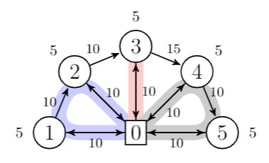
The new optimal routes are displayed below:
Time constraints
One may want to restrict the total duration of a route. In this case, a time attribute is set on each edge of the graph, and a maximum duration is set with prob.duration.
>>> for (u, v) in G.edges():
       G.edges[u,v]["time"] = 20
>>> G.edges[4,5]["time"] = 25
>>> prob.duration = 60
>>> prob.solve()
>>> prob.best_value
85.0
As the problem is more and more constrained, the total cost continues to increase. Lets check the durations of each route:
>>> prob.best_routes
{1: ["Source", 1, 2, "Sink"], 2: ["Source", 3, 4, "Sink"], 3: ["Source", 5, "Sink"]}
>>> prob.best_routes_duration
{1: 60, 2: 60, 3: 40}
The new optimal routes are displayed below:
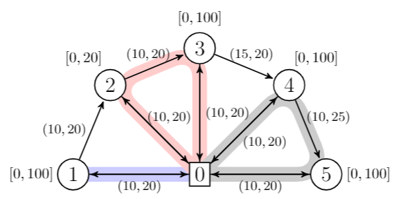
Time window constraints
When designing routes, it may be required that a customer is serviced in a given time window \([\ell,u]\). Such time windows are defined for each node, as well as service times.
>>> time_windows = {1: (5, 100), 2: (5, 20), 3: (5, 100), 4: (5, 100), 5: (5, 100)}
>>> for v in G.nodes():
        G.nodes[v]["lower"] = time_windows[v][0]
        G.nodes[v]["upper"] = time_windows[v][1]
        if v not in ["Source","Sink"]:
           G.nodes[v]["service_time"] = 1
A boolean parameter time_windows is activated to enforce
such constraints:
>>> prob.time_windows = True
>>> prob.duration = 64
>>> prob.solve()
>>> prob.best_value
90.0
The total cost increases again. Lets check the arrival times:
>>> prob.best_routes
{1: ["Source", 1, "Sink"], 4: ["Source", 2, 3, "Sink"], 2: ["Source", 4, "Sink"],  3: ["Source", 5, "Sink"]}
>>> prob.arrival_time
{1: {1: 20, 'Sink': 41}, 2: {4: 20, 'Sink': 41}, 3: {5: 20, 'Sink': 41}, 4: {2: 20, 3: 41, 'Sink': 62}}
The new optimal routes are displayed below:
Complete program
import networkx as nx
from vrpy import VehicleRoutingProblem

# Create graph
G = nx.DiGraph()
for v in [1, 2, 3, 4, 5]:
       G.add_edge("Source", v, cost=10, time=20)
   G.add_edge(v, "Sink", cost=10, time=20)
   G.nodes[v]["demand"] = 5
   G.nodes[v]["upper"] = 100
   G.nodes[v]["lower"] = 5
   G.nodes[v]["service_time"] = 1
G.nodes[2]["upper"] = 20
G.nodes["Sink"]["upper"] = 110
G.nodes["Source"]["upper"] = 100
G.add_edge(1, 2, cost=10, time=20)
G.add_edge(2, 3, cost=10, time=20)
G.add_edge(3, 4, cost=15, time=20)
G.add_edge(4, 5, cost=10, time=25)

# Create vrp
prob = VehicleRoutingProblem(G, num_stops=3, load_capacity=10, duration=64, time_windows=True)

# Solve and display solution
prob.solve()
print(prob.best_routes)
print(prob.best_value)
Periodic CVRP
For scheduling routes over a time period, one can define a frequency for each customer. For example, if over a planning period of two days, customer \(2\) must be visited twice, and the other customers only once:
>>> prob.periodic = 2
>>> G.nodes[2]["frequency"] = 2
>>> prob.solve()
>>> prob.best_routes
{1: ['Source', 1, 2, 'Sink'], 2: ['Source', 4, 5, 'Sink'], 3: ['Source', 2, 3, 'Sink']}
>>> prob.schedule
{0: [1, 2], 1: [3]}
We can see that customer \(2\) is visited on both days of the planning period (routes \(1\) and \(3\)), and that it is not visited more than once per day.
Mixed fleet
We end this small example with an illustration of the mixed_fleet option, when vehicles of different
types (capacities, travel costs, fixed costs) are operating.
The first vehicle has a load_capacity of \(5\) units, and no fixed_cost, while
the second vehicle has a load_capacity of \(20\) units, and a fixed_cost with value
\(5\). The travel costs of the second vehicle are \(1\) unit more expensive than
those of the first vehicle:
>>> from networkx import DiGraph
>>> from vrpy import VehicleRoutingProblem
>>> G = DiGraph()
>>> for v in [1, 2, 3, 4, 5]:
       G.add_edge("Source", v, cost=[10, 11])
       G.add_edge(v, "Sink", cost=[10, 11])
       G.nodes[v]["demand"] = 5
>>> G.add_edge(1, 2, cost=[10, 11])
>>> G.add_edge(2, 3, cost=[10, 11])
>>> G.add_edge(3, 4, cost=[15, 16])
>>> G.add_edge(4, 5, cost=[10, 11])
>>> prob=VehicleRoutingProblem(G, mixed_fleet=True, fixed_cost=[0, 5], load_capacity=[5, 20])
>>> prob.best_value
    85
>>> prob.best_routes
    {1: ['Source', 1, 'Sink'], 2: ['Source', 2, 3, 4, 5, 'Sink']}
>>> prob.best_routes_cost
    {1: 20, 2: 65}
>>> prob.best_routes_type
    {1: 0, 2: 1}
An example borrowed from ortools
We borrow this second example from the well known ortools [PF] routing library. We will use the data from the tutorial.
Network definition
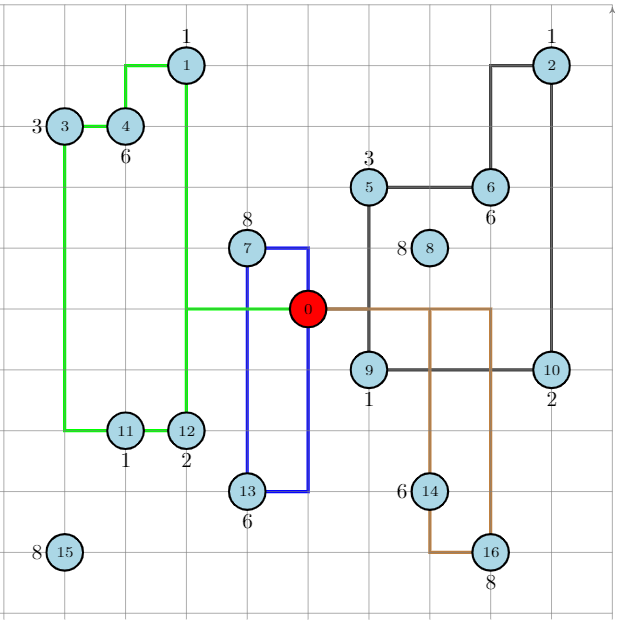
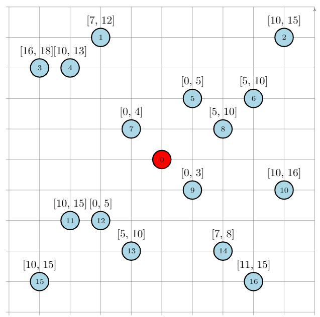
The graph is considered complete, that is, there are edges between each pair of nodes, in both directions, and the cost on each edge is defined as the Manhattan distance between both endpoints. The network is displayed below (for readability, edges are not shown), with the depot in red, and the labels outside of the vertices are the demands:
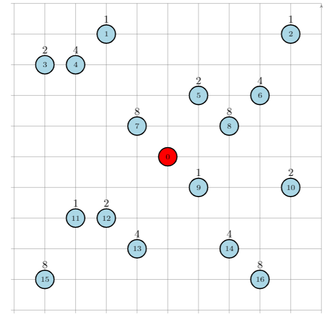
The network can be entirely defined by its distance matrix. We will make use of the NetworkX module to create this graph and store its attributes:
from networkx import DiGraph, from_numpy_matrix, relabel_nodes, set_node_attributes
from numpy import array

# Distance matrix
DISTANCES = [
[0,548,776,696,582,274,502,194,308,194,536,502,388,354,468,776,662,0], # from Source
[0,0,684,308,194,502,730,354,696,742,1084,594,480,674,1016,868,1210,548],
[0,684,0,992,878,502,274,810,468,742,400,1278,1164,1130,788,1552,754,776],
[0,308,992,0,114,650,878,502,844,890,1232,514,628,822,1164,560,1358,696],
[0,194,878,114,0,536,764,388,730,776,1118,400,514,708,1050,674,1244,582],
[0,502,502,650,536,0,228,308,194,240,582,776,662,628,514,1050,708,274],
[0,730,274,878,764,228,0,536,194,468,354,1004,890,856,514,1278,480,502],
[0,354,810,502,388,308,536,0,342,388,730,468,354,320,662,742,856,194],
[0,696,468,844,730,194,194,342,0,274,388,810,696,662,320,1084,514,308],
[0,742,742,890,776,240,468,388,274,0,342,536,422,388,274,810,468,194],
[0,1084,400,1232,1118,582,354,730,388,342,0,878,764,730,388,1152,354,536],
[0,594,1278,514,400,776,1004,468,810,536,878,0,114,308,650,274,844,502],
[0,480,1164,628,514,662,890,354,696,422,764,114,0,194,536,388,730,388],
[0,674,1130,822,708,628,856,320,662,388,730,308,194,0,342,422,536,354],
[0,1016,788,1164,1050,514,514,662,320,274,388,650,536,342,0,764,194,468],
[0,868,1552,560,674,1050,1278,742,1084,810,1152,274,388,422,764,0,798,776],
[0,1210,754,1358,1244,708,480,856,514,468,354,844,730,536,194,798,0,662],
[0,0,0,0,0,0,0,0,0,0,0,0,0,0,0,0,0,0], # from Sink
]

# Demands (key: node, value: amount)
DEMAND = {1: 1, 2: 1, 3: 2, 4: 4, 5: 2, 6: 4, 7: 8, 8: 8, 9: 1, 10: 2, 11: 1, 12: 2, 13: 4, 14: 4, 15: 8, 16: 8}

# The matrix is transformed into a DiGraph
A = array(DISTANCES, dtype=[("cost", int)])
G = from_numpy_matrix(A, create_using=nx.DiGraph())

# The demands are stored as node attributes
set_node_attributes(G, values=DEMAND, name="demand")

# The depot is relabeled as Source and Sink
G = relabel_nodes(G, {0: "Source", 17: "Sink"})
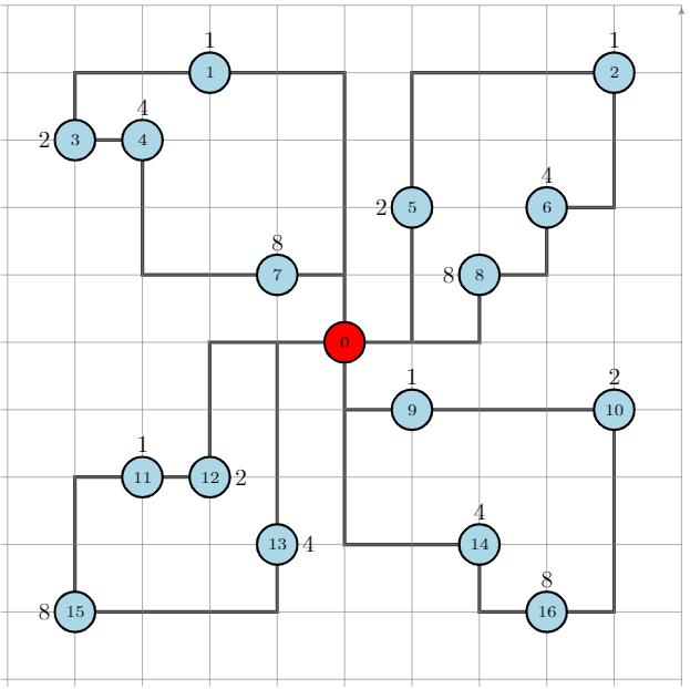
CVRP
Once the graph is properly defined, creating a CVRP and solving it is straightforward. With a maximum load of \(15\) units per vehicle:
>>> from vrpy import VehicleRoutingProblem
>>> prob = VehicleRoutingProblem(G, load_capacity=15)
>>> prob.solve()
>>> prob.best_value
6208.0
>>> prob.best_routes
{1: ['Source', 12, 11, 15, 13, 'Sink'], 2: ['Source', 1, 3, 4, 7, 'Sink'], 3: ['Source', 5, 2, 6, 8, 'Sink'], 4: ['Source', 14, 16, 10, 9, 'Sink']}
>>> prob.best_routes_load
{1: 15, 2: 15, 3: 15, 4: 15}
The four routes are displayed below:
CVRP with simultaneous distribution and collection
We follow with the exact same configuration, but this time, every time a node is visited, the vehicle unloads its demand and loads some waste material.
from networkx import DiGraph, from_numpy_matrix, relabel_nodes, set_node_attributes
from numpy import array

# Distance matrix
DISTANCES = [
[0,548,776,696,582,274,502,194,308,194,536,502,388,354,468,776,662,0], # from Source
[0,0,684,308,194,502,730,354,696,742,1084,594,480,674,1016,868,1210,548],
[0,684,0,992,878,502,274,810,468,742,400,1278,1164,1130,788,1552,754,776],
[0,308,992,0,114,650,878,502,844,890,1232,514,628,822,1164,560,1358,696],
[0,194,878,114,0,536,764,388,730,776,1118,400,514,708,1050,674,1244,582],
[0,502,502,650,536,0,228,308,194,240,582,776,662,628,514,1050,708,274],
[0,730,274,878,764,228,0,536,194,468,354,1004,890,856,514,1278,480,502],
[0,354,810,502,388,308,536,0,342,388,730,468,354,320,662,742,856,194],
[0,696,468,844,730,194,194,342,0,274,388,810,696,662,320,1084,514,308],
[0,742,742,890,776,240,468,388,274,0,342,536,422,388,274,810,468,194],
[0,1084,400,1232,1118,582,354,730,388,342,0,878,764,730,388,1152,354,536],
[0,594,1278,514,400,776,1004,468,810,536,878,0,114,308,650,274,844,502],
[0,480,1164,628,514,662,890,354,696,422,764,114,0,194,536,388,730,388],
[0,674,1130,822,708,628,856,320,662,388,730,308,194,0,342,422,536,354],
[0,1016,788,1164,1050,514,514,662,320,274,388,650,536,342,0,764,194,468],
[0,868,1552,560,674,1050,1278,742,1084,810,1152,274,388,422,764,0,798,776],
[0,1210,754,1358,1244,708,480,856,514,468,354,844,730,536,194,798,0,662],
[0,0,0,0,0,0,0,0,0,0,0,0,0,0,0,0,0,0], # from Sink
]

# Delivery demands (key: node, value: amount)
DEMAND = {1: 1, 2: 1, 3: 2, 4: 4, 5: 2, 6: 4, 7: 8, 8: 8, 9: 1, 10: 2, 11: 1, 12: 2, 13: 4, 14: 4, 15: 8, 16: 8}

# Pickup waste (key: node, value: amount)
COLLECT = {1: 1, 2: 1, 3: 1, 4: 1, 5: 2, 6: 1, 7: 4, 8: 1, 9: 1, 10: 2, 11: 3, 12: 2, 13: 4, 14: 2, 15: 1, 16: 2}

# The matrix is transformed into a DiGraph
A = array(DISTANCES, dtype=[("cost", int)])
G = from_numpy_matrix(A, create_using=nx.DiGraph())

# The distribution and collection amounts are stored as node attributes
set_node_attributes(G, values=DEMAND, name="demand")
set_node_attributes(G, values=COLLECT, name="collect")

# The depot is relabeled as Source and Sink
G = relabel_nodes(G, {0: "Source", 17: "Sink"})
The load_capacity is unchanged, and the distribution_collection attribute is set to True.
>>> from vrpy import VehicleRoutingProblem
>>> prob = VehicleRoutingProblem(G, load_capacity=15, distribution_collection=True)
>>> prob.solve()
    >>> prob.best_value
6208.0
>>> prob.best_routes
{1: ['Source', 12, 11, 15, 13, 'Sink'], 2: ['Source', 1, 3, 4, 7, 'Sink'], 3: ['Source', 5, 2, 6, 8, 'Sink'], 4: ['Source', 14, 16, 10, 9, 'Sink']}
>>> prob.node_load
{1: {7: 4, 3: 5, 4: 8, 1: 8, 'Sink': 8}, 2: {8: 7, 6: 10, 2: 10, 5: 10, 'Sink': 10}, 3: {14: 2, 16: 8, 10: 8, 9: 8, 'Sink': 8}, 4: {13: 0, 15: 7, 11: 5, 12: 5, 'Sink': 5}}
The optimal solution is unchanged. This is understandable, as for each node, the distribution volume is greater than (or equals) the pickup volume.
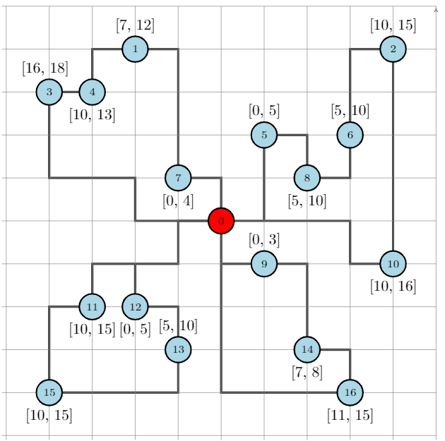
VRP with time windows
Each node must now be serviced within a time window. The time windows are displayed above each node:
This time, the network is defined by its distance matrix and its time matrix:
from networkx import DiGraph, from_numpy_matrix, relabel_nodes, set_node_attributes
from numpy import array

# Distance matrix
DISTANCES = [
     [0,548,776,696,582,274,502,194,308,194,536,502,388,354,468,776,662,0], # from Source
     [0,0,684,308,194,502,730,354,696,742,1084,594,480,674,1016,868,1210,548],
     [0,684,0,992,878,502,274,810,468,742,400,1278,1164,1130,788,1552,754,776],
     [0,308,992,0,114,650,878,502,844,890,1232,514,628,822,1164,560,1358,696],
     [0,194,878,114,0,536,764,388,730,776,1118,400,514,708,1050,674,1244,582],
     [0,502,502,650,536,0,228,308,194,240,582,776,662,628,514,1050,708,274],
     [0,730,274,878,764,228,0,536,194,468,354,1004,890,856,514,1278,480,502],
     [0,354,810,502,388,308,536,0,342,388,730,468,354,320,662,742,856,194],
     [0,696,468,844,730,194,194,342,0,274,388,810,696,662,320,1084,514,308],
     [0,742,742,890,776,240,468,388,274,0,342,536,422,388,274,810,468,194],
     [0,1084,400,1232,1118,582,354,730,388,342,0,878,764,730,388,1152,354,536],
     [0,594,1278,514,400,776,1004,468,810,536,878,0,114,308,650,274,844,502],
     [0,480,1164,628,514,662,890,354,696,422,764,114,0,194,536,388,730,388],
     [0,674,1130,822,708,628,856,320,662,388,730,308,194,0,342,422,536,354],
     [0,1016,788,1164,1050,514,514,662,320,274,388,650,536,342,0,764,194,468],
     [0,868,1552,560,674,1050,1278,742,1084,810,1152,274,388,422,764,0,798,776],
     [0,1210,754,1358,1244,708,480,856,514,468,354,844,730,536,194,798,0,662],
     [0,0,0,0,0,0,0,0,0,0,0,0,0,0,0,0,0,0], # from Sink
     ]

TRAVEL_TIMES = [
    [0, 6, 9, 8, 7, 3, 6, 2, 3, 2, 6, 6, 4, 4, 5, 9, 7, 0],  # from source
    [0, 0, 8, 3, 2, 6, 8, 4, 8, 8, 13, 7, 5, 8, 12, 10, 14, 6],
    [0, 8, 0, 11, 10, 6, 3, 9, 5, 8, 4, 15, 14, 13, 9, 18, 9, 9],
    [0, 3, 11, 0, 1, 7, 10, 6, 10, 10, 14, 6, 7, 9, 14, 6, 16, 8],
    [0, 2, 10, 1, 0, 6, 9, 4, 8, 9, 13, 4, 6, 8, 12, 8, 14, 7],
    [0, 6, 6, 7, 6, 0, 2, 3, 2, 2, 7, 9, 7, 7, 6, 12, 8, 3],
    [0, 8, 3, 10, 9, 2, 0, 6, 2, 5, 4, 12, 10, 10, 6, 15, 5, 6],
    [0, 4, 9, 6, 4, 3, 6, 0, 4, 4, 8, 5, 4, 3, 7, 8, 10, 2],
    [0, 8, 5, 10, 8, 2, 2, 4, 0, 3, 4, 9, 8, 7, 3, 13, 6, 3],
    [0, 8, 8, 10, 9, 2, 5, 4, 3, 0, 4, 6, 5, 4, 3, 9, 5, 2],
    [0, 13, 4, 14, 13, 7, 4, 8, 4, 4, 0, 10, 9, 8, 4, 13, 4, 6],
    [0, 7, 15, 6, 4, 9, 12, 5, 9, 6, 10, 0, 1, 3, 7, 3, 10, 6],
    [0, 5, 14, 7, 6, 7, 10, 4, 8, 5, 9, 1, 0, 2, 6, 4, 8, 4],
    [0, 8, 13, 9, 8, 7, 10, 3, 7, 4, 8, 3, 2, 0, 4, 5, 6, 4],
    [0, 12, 9, 14, 12, 6, 6, 7, 3, 3, 4, 7, 6, 4, 0, 9, 2, 5],
    [0, 10, 18, 6, 8, 12, 15, 8, 13, 9, 13, 3, 4, 5, 9, 0, 9, 9],
    [0, 14, 9, 16, 14, 8, 5, 10, 6, 5, 4, 10, 8, 6, 2, 9, 0, 7],
    [0, 0, 0, 0, 0, 0, 0, 0, 0, 0, 0, 0, 0, 0, 0, 0, 0, 0],  # from sink
    ]

# Time windows (key: node, value: lower/upper bound)
TIME_WINDOWS_LOWER = {0: 0, 1: 7, 2: 10, 3: 16, 4: 10, 5: 0, 6: 5, 7: 0, 8: 5, 9: 0, 10: 10, 11: 10, 12: 0, 13: 5, 14: 7, 15: 10, 16: 11,}
TIME_WINDOWS_UPPER = {1: 12, 2: 15, 3: 18, 4: 13, 5: 5, 6: 10, 7: 4, 8: 10, 9: 3, 10: 16, 11: 15, 12: 5, 13: 10, 14: 8, 15: 15, 16: 15,}

# Transform distance matrix into DiGraph
A = array(DISTANCES, dtype=[("cost", int)])
G_d = from_numpy_matrix(A, create_using=DiGraph())

# Transform time matrix into DiGraph
A = array(TRAVEL_TIMES, dtype=[("time", int)])
G_t = from_numpy_matrix(A, create_using=DiGraph())

# Merge
G = compose(G_d, G_t)

# Set time windows
set_node_attributes(G, values=TIME_WINDOWS_LOWER, name="lower")
set_node_attributes(G, values=TIME_WINDOWS_UPPER, name="upper")

# The VRP is defined and solved
prob = VehicleRoutingProblem(G, time_windows=True)
prob.solve()
The solution is displayed below:
>>> prob.best_value
    6528.0
>>> prob.best_routes
    {1: ['Source', 9, 14, 16, 'Sink'], 2: ['Source', 12, 13, 15, 11, 'Sink'], 3: ['Source', 5, 8, 6, 2, 10, 'Sink'], 4: ['Source', 7, 1, 4, 3, 'Sink']}
>>> prob.arrival_time
    {1: {9: 2, 14: 7, 16: 11, 'Sink': 18}, 2: {12: 4, 13: 6, 15: 11, 11: 14, 'Sink': 20}, 3: {5: 3, 8: 5, 6: 7, 2: 10, 10: 14, 'Sink': 20}, 4: {7: 2, 1: 7, 4: 10, 3: 16, 'Sink': 24}}
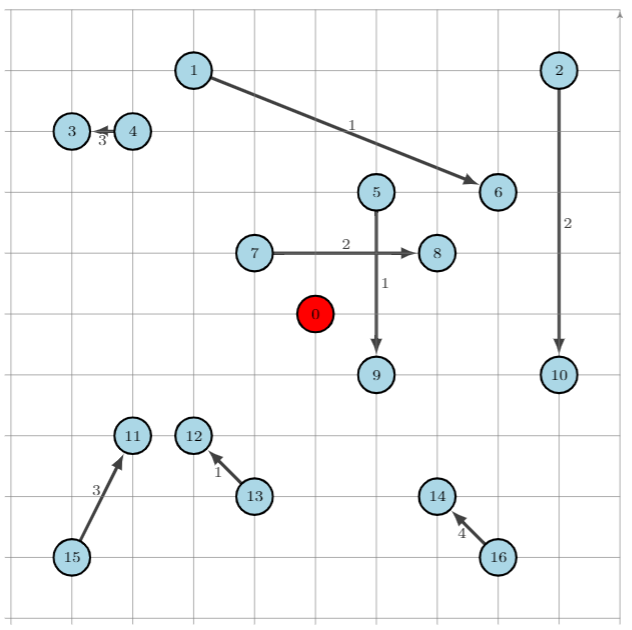
CVRP with pickups and deliveries
In this variant, each demand is made of a pickup node and a delivery node. Each pickup/delivery pair (or request) must be assigned to the same tour, and within this tour, the pickup node must be visited prior to the delivery node (as an item that is yet to be picked up cannot be delivered). The total load must not exceed the vehicle’s capacity. The requests are displayed below:
The network is defined as previously, and we add the following data to take into account each request:
# Requests (from_node, to_node) : amount
pickups_deliveries = {(1, 6): 1, (2, 10): 2, (4, 3): 3, (5, 9): 1, (7, 8): 2, (15, 11): 3, (13, 12): 1, (16, 14): 4}
for (u, v) pickups_deliveries:
    G.nodes[u]["request"] = v
    # Pickups are accounted for positively
    G.nodes[u]["demand"] = pickups_deliveries[(u, v)]
    # Deliveries are accounted for negatively
    G.nodes[v]["demand"] = -pickups_deliveries[(u, v)]
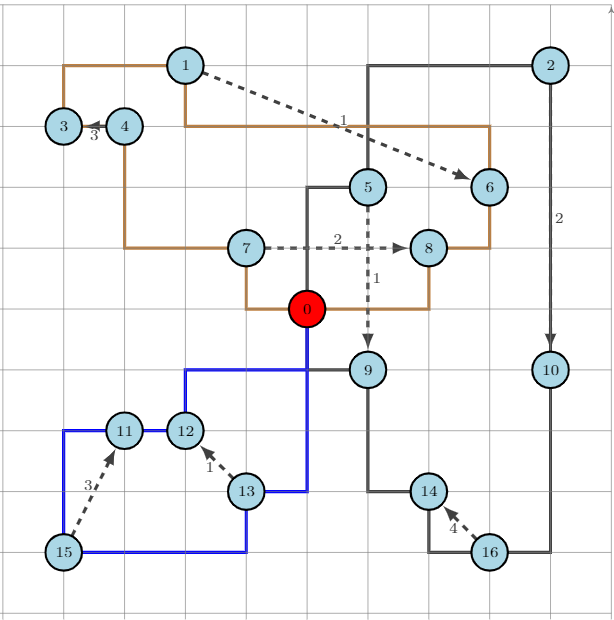
We can now create a pickup and delivery instance with a maximum load of \(6\) units per vehicle, and with at most \(6\) stops:
>>> from vrpy import VehicleRoutingProblem
>>> prob = VehicleRoutingProblem(G, load_capacity=6, num_stops=6, pickup_delivery=True)
>>> prob.solve(cspy=False)
>>> prob.best_value
5980.0
>>> prob.best_routes
{1: ['Source', 5, 2, 10, 16, 14, 9, 'Sink'], 2: ['Source', 7, 4, 3, 1, 6, 8, 'Sink'], 3: ['Source', 13, 15, 11, 12, 'Sink']}
>>> prob.node_load
{1: {5: 1, 2: 3, 10: 1, 16: 5, 14: 1, 9: 0, 'Sink': 0}, 2: {7: 2, 4: 5, 3: 2, 1: 3, 6: 2, 8: 0, 'Sink': 0}, 3: {13: 1, 15: 4, 11: 1, 12: 0, 'Sink': 0}}
The four routes are displayed below:
Limited fleet and dropping visits
This last example is similar to the above CVRP, except for the fact that demands have increased, and that the fleet is limited to \(4\) vehicles, with a \(15\) unit capacity (per vehicle). Since the total demand is greater than \(4 \times 15 = 60\), servicing each node is not possible, therefore, we will try to visit as many customers as possible, and allow dropping visits, at the cost of a \(1000\) penalty.
from networkx import DiGraph, from_numpy_matrix, relabel_nodes, set_node_attributes
from numpy import array

# Distance matrix
DISTANCES = [
[0,548,776,696,582,274,502,194,308,194,536,502,388,354,468,776,662,0], # from Source
[0,0,684,308,194,502,730,354,696,742,1084,594,480,674,1016,868,1210,548],
[0,684,0,992,878,502,274,810,468,742,400,1278,1164,1130,788,1552,754,776],
[0,308,992,0,114,650,878,502,844,890,1232,514,628,822,1164,560,1358,696],
[0,194,878,114,0,536,764,388,730,776,1118,400,514,708,1050,674,1244,582],
[0,502,502,650,536,0,228,308,194,240,582,776,662,628,514,1050,708,274],
[0,730,274,878,764,228,0,536,194,468,354,1004,890,856,514,1278,480,502],
[0,354,810,502,388,308,536,0,342,388,730,468,354,320,662,742,856,194],
[0,696,468,844,730,194,194,342,0,274,388,810,696,662,320,1084,514,308],
[0,742,742,890,776,240,468,388,274,0,342,536,422,388,274,810,468,194],
[0,1084,400,1232,1118,582,354,730,388,342,0,878,764,730,388,1152,354,536],
[0,594,1278,514,400,776,1004,468,810,536,878,0,114,308,650,274,844,502],
[0,480,1164,628,514,662,890,354,696,422,764,114,0,194,536,388,730,388],
[0,674,1130,822,708,628,856,320,662,388,730,308,194,0,342,422,536,354],
[0,1016,788,1164,1050,514,514,662,320,274,388,650,536,342,0,764,194,468],
[0,868,1552,560,674,1050,1278,742,1084,810,1152,274,388,422,764,0,798,776],
[0,1210,754,1358,1244,708,480,856,514,468,354,844,730,536,194,798,0,662],
[0,0,0,0,0,0,0,0,0,0,0,0,0,0,0,0,0,0], # from Sink
]

# Demands (key: node, value: amount)
DEMAND = {1: 1, 2: 1, 3: 3, 4: 6, 5: 3, 6: 6, 7: 8, 8: 8, 9: 1, 10: 2, 11: 1, 12: 2, 13: 6, 14: 6, 15: 8, 16: 8}

# The matrix is transformed into a DiGraph
A = array(DISTANCES, dtype=[("cost", int)])
G = from_numpy_matrix(A, create_using=nx.DiGraph())

# The demands are stored as node attributes
set_node_attributes(G, values=DEMAND, name="demand")

# The depot is relabeled as Source and Sink
G = relabel_nodes(G, {0: "Source", 17: "Sink"})
Once the graph is properly defined, a VRP instance is created, with attributes num_vehicles and drop_penalty:
>>> from vrpy import VehicleRoutingProblem
>>> prob = VehicleRoutingProblem(G, load_capacity=15, num_vehicles=4, drop_penalty=1000)
>>> prob.solve()
>>> prob.best_value
7776.0
>>> prob.best_routes
{1: ['Source', 9, 10, 2, 6, 5, 'Sink'], 2: ['Source', 7, 13, 'Sink'], 3: ['Source', 14, 16, 'Sink'], 4: ['Source', 1, 4, 3, 11, 12, 'Sink']}
>>> prob.best_routes_load
{1: 13, 2: 14, 3: 14, 4: 13}
The solver drops nodes \(8\) and \(15\). The new optimal routes are displayed below: